
Most traders never actually know whether their strategy works. They know how the last three trades felt. They know the one screenshot they posted when it ripped. They know the vague sense that "this setup usually works." And on the strength of that feeling, they size up — right into the drawdown that finally teaches them the feeling was never evidence.
This guide is about replacing the feeling with a number. Not because numbers are magic, but because a number can be tested, compared, and trusted in a way a memory never can. A memory is edited by hope. A memory keeps the winners in high definition and lets the losers go blurry. A number does neither. By the end of this piece you'll be able to take any setup you trade — a 55-EMA reclaim, a golden-pocket bounce, an opening-range break, a failed breakdown at the prior-day low — and answer the only question that matters before you increase risk: does this actually make money over a large sample, or does it just feel like it does?
We're going to build this from the ground up and leave nothing hand-wavy. Win rate and reward-to-risk, and why neither one alone means anything. The expectancy formula that ties them together into a single verdict. How many trades you need before that verdict is real, and the actual variance math behind that answer. How the whole picture changes in a trending market versus a chop-fest versus a high-volatility panic. How to layer expectancy across timeframes, and how to combine it with two or three other tools so it sharpens your read instead of replacing it. How to forward-test without lying to yourself. And the curve-fitting traps that make a garbage strategy look like a money printer on a backtest and then bleed you dry live. Worked numbers throughout — because this is a subject where hand-waving is exactly how people lose money.
The Concept: An Edge Is a Positive Average, Not a Winning Trade
Let's define the core term once and carry it the whole way through. An edge is a statistical tendency for your trades, taken as a group, to make more than they lose over a large number of repetitions. That's it. An edge is not a good trade. It's not a winning streak. It's not being right about direction. It's a positive average outcome per trade, proven across enough trades that luck can't explain it.
This distinction is the whole game, so sit with it. A single trade tells you almost nothing about whether you have an edge, the same way a single coin flip tells you nothing about whether a coin is fair. You can flip a fair coin and get five heads in a row. You can take a genuinely bad setup and win four times before it turns on you. The outcome of any one trade is dominated by randomness — what the market happened to do in the next few hours. The edge only shows up in the aggregate, when you've repeated the setup enough times that the randomness averages out and the underlying tendency is left standing.
The casino is the cleanest mental model here, and it's worth holding onto for the rest of this guide. A casino has roughly a 5% edge on roulette. On any single spin, the casino can lose — and lose big. On any single night, one table can bleed. The casino does not care, and it does not change the rules after a bad night, because it knows two things the average trader does not: the edge is small, and the edge is certain to express itself over tens of thousands of spins. The casino's entire business is not winning any given bet. It's getting enough repetitions of a small edge that variance becomes irrelevant. That is exactly the business you are in. Your setup is the wheel. Your job is to know your number and take the spins.
So the first mental shift: stop grading yourself on trades and start grading yourself on processes repeated many times. A trade can lose and still have been the correct, positive-edge decision. A trade can win and still have been a reckless, negative-edge gamble that happened to pay. If you can't separate the quality of the decision from the outcome of the roll, everything downstream in this guide will be invisible to you, because you'll keep promoting lucky gambles and retiring unlucky edges.
There's a useful four-box here that professional desks think in constantly. Every trade lands in one of four cells: good decision + win, good decision + loss, bad decision + win, bad decision + loss. Two of those cells are easy — good/win feels great, bad/loss feels bad, and both are correctly labeled by the outcome. The two that destroy accounts are the diagonal. Good decision + loss is the trade beginners abandon and pros repeat. Bad decision + win is the trade beginners repeat and pros flag as dangerous. The single most expensive habit in trading is letting the outcome of a trade relabel the quality of the decision. Expectancy is the tool that lets you grade the decision directly, on its own long-run merit, so a green day never talks you into a bad process and a red day never talks you out of a good one.
The tool that lets you measure a process instead of a trade is expectancy — the average dollars (or R, or points) you can expect to make per trade over the long run. Everything else in this piece exists to compute that number honestly, and to know when you're allowed to believe it.
The Mechanism, Part 1: Win Rate and R:R Are Two Dials, Not One
Two numbers describe any strategy's raw performance, and the single most common beginner mistake is caring about only the first one.
Win rate is the percentage of your trades that make money. Win 55 out of 100 trades, your win rate is 55%. Simple, and seductive — it feels like the measure of whether you're good. It isn't. It's half of the measure, and on its own it's the less important half.
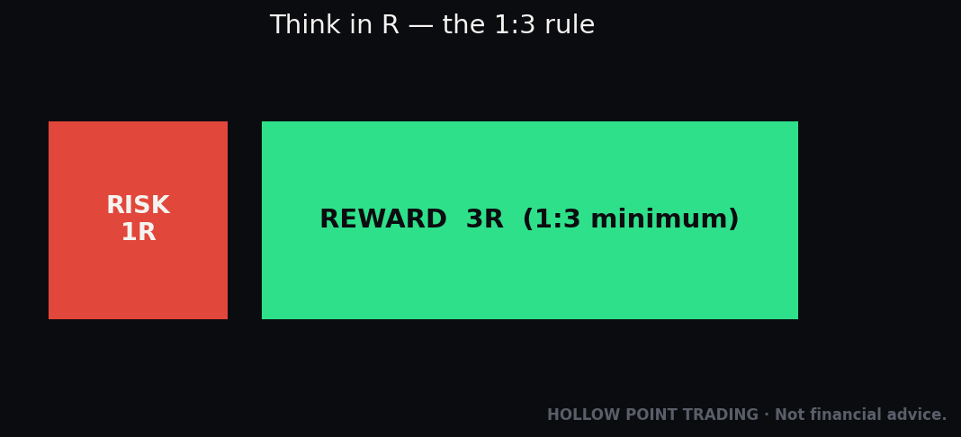
Reward-to-risk ratio, written R:R, is how much you make on a winner compared to how much you lose on a loser. If you risk $100 to make $300, that's 3:1 — three units of reward for one unit of risk. HPT builds every trade around a minimum of 1:3 R/R for exactly the reason we're about to make numerical.
Here's why win rate alone is a trap. Imagine two traders.
Trader A wins 80% of the time. Sounds elite. But she's a chronic profit-taker who snatches $50 winners and lets losers run to $400 before she gives up. Over 10 trades she wins 8 (+$50 each = +$400) and loses 2 (−$400 each = −$800). Net: −$400. An 80% win rate, and she's losing money.
Trader B wins 35% of the time. Sounds terrible. But he risks $100 to make $400, cuts losers fast, and lets winners run. Over 10 trades he wins 3.5 (+$400 each = +$1,400) and loses 6.5 (−$100 each = −$650). Net: +$750. A 35% win rate, and he's the one printing.
Win rate and R:R are two dials on the same machine. Turn one up and you can usually turn the other down — high win-rate strategies tend to have small R:R (you take profits early and often), and high-R:R strategies tend to have low win rates (you're swinging for the fences and missing a lot). What matters is the combination, and the formula that combines them is expectancy.
The breakeven line: the cheat you can do in your head
Before we even get to the full formula, there's a shortcut that pays for itself daily. For any reward-to-risk ratio, there is a breakeven win rate — the win rate at which the strategy makes exactly zero. The formula is dead simple:
Breakeven Win% = 1 / (1 + R:R)
At 1:1 R:R, breakeven win rate is 1/2 = 50%. Makes sense — if wins and losses are the same size, you need to win half the time to tread water. At 1:2, it's 1/3 = 33%. At 1:3, it's 1/4 = 25%. At 1:4, it's 1/5 = 20%. This is the number you carry in your head all day. If you trade an HPT setup at a genuine 1:3 and you win more than 25% of the time, you make money. Full stop. The 40% win rate that feels like failure is a full 15 points above breakeven — an enormous margin.
Flip it and it exposes Trader A instantly. Her R:R is roughly 50:400, or 1:8 against her — she risks eight units to make one. Her breakeven win rate is 1/(1 + 0.125) = 89%. She wins 80%. She is nine points below the line she'd need, which is exactly why an 80% win rate loses her money. You didn't need the full expectancy formula to smell the problem; the breakeven line caught it in one step.
Keep four of these memorized and you'll never again be seduced by a win-rate number in isolation: 1:1 needs 50%, 1:2 needs 33%, 1:3 needs 25%, 1:4 needs 20%. Every time someone brags about a win rate, your first silent question becomes "at what R:R?" — and their number stops meaning anything until they answer it.
The Mechanism, Part 2: The Expectancy Formula
Here is the equation that turns two dials into one verdict:
Expectancy = (Win% × Average Win) − (Loss% × Average Loss)
In words: take what you make on your winners, weighted by how often you win. Subtract what you lose on your losers, weighted by how often you lose. What's left is the average outcome of a single trade — your edge, expressed in dollars.
Let's run Trader B through it. Win% = 0.35, average win = $400. Loss% = 0.65, average loss = $100.
Expectancy = (0.35 × $400) − (0.65 × $100) = $140 − $65 = +$75 per trade.
That +$75 is the number that actually matters. It says: every time this trader takes this setup, on average, he pockets $75 — even though he's wrong most of the time. Take the setup 200 times a year and that's $15,000 of expectancy, before you've said a word about whether any individual trade won.
Now Trader A. Win% = 0.80, average win = $50. Loss% = 0.20, average loss = $400.
Expectancy = (0.80 × $50) − (0.20 × $400) = $40 − $80 = −$40 per trade.
Every time she takes her setup, she loses $40 on average. The 80% win rate is a decoration on a losing machine. This is why "what's your win rate" is the wrong first question, and "what's your expectancy" is the right one.
Expressing expectancy in R
Dollars depend on your position size, which changes. A cleaner, size-independent way to talk about expectancy is in R, where 1R is the amount you risk on a trade. If you always risk $100, then a $300 winner is +3R and a full stop-out is −1R.
Restate the formula in R. For Trader B, winners are +4R, losers are −1R:
Expectancy = (0.35 × 4R) − (0.65 × 1R) = 1.4R − 0.65R = +0.75R per trade.
Now the number travels. Whether you're trading a $500 account or a $500,000 account, a setup with +0.75R expectancy makes you three-quarters of your risk unit per trade on average. This is the language to think in, because it lets you compare a scalp and a swing on the same scale, and it makes position sizing a separate decision from edge — which is exactly how it should be. Find the edge first in R. Decide how many dollars 1R is second.
The messy real-world version: partial wins, trailed stops, and scratches
The textbook formula assumes every winner is exactly +3R and every loser is exactly −1R. Real trading is grainier than that. You trail a stop and a "winner" closes at +1.4R. You take a runner and it hits +5.2R. You get shaken at breakeven for +0.1R. Two losers gap through your stop and cost −1.4R and −1.2R instead of a clean −1R. When your outcomes are a spray of different R-values, don't force them into the two-bucket formula — just use the general expectancy definition, which is simply the average of every trade's R result:
Expectancy (R) = (sum of all trade R-multiples) ÷ (number of trades)
Say you log ten trades with these R outcomes: +3.0, −1.0, +1.4, −1.0, +5.2, −1.0, +0.1, −1.2, −1.0, +2.8. Add them: 3.0 − 1.0 + 1.4 − 1.0 + 5.2 − 1.0 + 0.1 − 1.2 − 1.0 + 2.8 = +6.3R total. Divide by 10 trades = +0.63R per trade. That's your real expectancy, and it already bakes in the trailing, the scratches, and the slippage on the two ugly losers, because you used the actual R each trade produced. This is the version you'll use most in practice; the two-bucket formula is really just a teaching simplification of this one.
A quick reference for what these numbers mean: expectancy above 0 means the setup makes money over a large sample. Below 0 means it loses, no matter how good it feels. And a rough professional benchmark — anything north of +0.2R to +0.3R per trade, held with discipline across a real sample, is a genuinely tradeable edge. You do not need +2R monsters. You need a small positive number you can repeat a thousand times. A desk running +0.3R expectancy at 400 trades a year is compounding +120R annually — that is a career, not a lottery ticket.
Expectancy per unit of time, not just per trade
One refinement the pros make and beginners miss: two setups with identical per-trade expectancy are not equally valuable if one fires ten times as often. A swing setup at +0.8R that triggers 20 times a year produces +16R annually. A scalp at +0.25R that triggers 300 times a year produces +75R annually — nearly five times the total edge — despite being the "worse" setup on a per-trade basis. This is expectancy density: expectancy per trade multiplied by trade frequency, which tells you the total R a setup can actually contribute to your year. Frequency is a multiplier on edge. A tiny edge you can take often can outproduce a fat edge that barely shows up — provided, and this matters enormously, the frequent setup survives costs, which we'll get to.
The Mechanism, Part 3: Sample Size and Variance
Now the part almost everyone skips, and the part that separates people who know they have an edge from people who hope they do.
You computed Trader B's expectancy at +0.75R. But you computed it from a win rate of 35% and a specific average win. Where did those come from? If they came from 12 trades, they're worthless. If they came from 300 trades, now we're talking. The reason is variance — the natural, random spread of outcomes around the true average.
Think back to the coin. A fair coin's true heads rate is 50%. But flip it 10 times and you might easily see 7 heads (70%) or 3 heads (30%). The measured rate swings wildly around the true rate when the sample is small. Flip it 1,000 times and you'll be hugging 50% — say, between 47% and 53%. The measured rate converges on the truth only as the sample grows. This is the law of large numbers, and it is the single most important idea in judging a strategy.
Your backtest win rate is a coin-flip measurement. A setup with a true win rate of 40% can easily show 55% over 20 trades purely by luck, or show 25% over 20 trades and make you abandon a perfectly good edge. Twenty trades tells you almost nothing. This is why the trader who says "I tried it, took eight trades, lost money, it doesn't work" has learned exactly nothing about the strategy and everything about their own impatience.
How big does the sample need to be?
There's no single magic number, but here are working rules you can actually use.
Minimum to form any opinion: ~30 trades. Below this you're reading noise. Around 30, the math starts to stabilize enough for a first, heavily-caveated read. Treat any conclusion here as a pencil sketch, not ink.
A real read: 100+ trades. This is where most retail-scale edges become believable. At 100 trades the random error in your win rate roughly halves compared to 25, and a genuinely positive expectancy usually stops hiding.
A confident read: 200–300+ trades. For lower win-rate, high-R:R strategies especially — where a few big winners drive everything — you need more trades, because the outcome depends on catching those rare winners a representative number of times.
Here's the intuition for why low win-rate strategies need bigger samples. If your edge comes from 3-in-10 trades that each pay +4R, then whether you're up or down over 20 trades depends almost entirely on whether you happened to catch 4 of those winners or only 2. Miss the rare payoff by a couple of instances and a great strategy looks broken. The rarer the event that carries your edge, the larger the sample you need before the average is trustworthy. A 65%-win-rate scalp stabilizes faster than a 30%-win-rate runner strategy, even though both may have identical expectancy, because the scalp's outcome doesn't hinge on rare fat-tail wins.
A variance gut-check you can do in your head
Take your win rate as a decimal, call it p. A rough one-standard-deviation swing in your measured win rate over N trades is √(p×(1−p)/N). For a 40% strategy over 25 trades: √(0.4×0.6/25) = √0.0096 ≈ 0.098, about 10 points. So your "40% strategy" can routinely measure anywhere from 30% to 50% over 25 trades on luck alone. Push N to 200 and that swing drops to about 3.5 points — 36.5% to 43.5%. That's the difference sample size makes, and it's why the same setup can look like a winner and a loser to two traders who each took it a dozen times.
Notice the shape of that math: to halve your uncertainty you have to quadruple your sample, because N sits under a square root. Going from 25 to 100 trades halves the error band. Going from 100 to 400 halves it again. This is why the last bit of confidence is so expensive to buy, and why chasing a perfectly certain edge is a fool's errand. You are never aiming for certainty. You are aiming for enough sample that the pessimistic end of your estimate still clears the bar.
The drawdown you must survive to collect the edge
Sample size has a second, more visceral consequence that pure win-rate math hides: losing streaks are longer than your gut expects, even in a great strategy. A 40%-win-rate setup loses 60% of the time. The probability of n losses in a row is 0.6ⁿ. Six straight losses has probability 0.6⁶ ≈ 4.7% — which sounds rare until you realize that across 200 trades, a streak of six or more losers is not just possible, it is nearly certain to happen at least once. Eight in a row (0.6⁸ ≈ 1.7%) will show up in a long enough sample too.
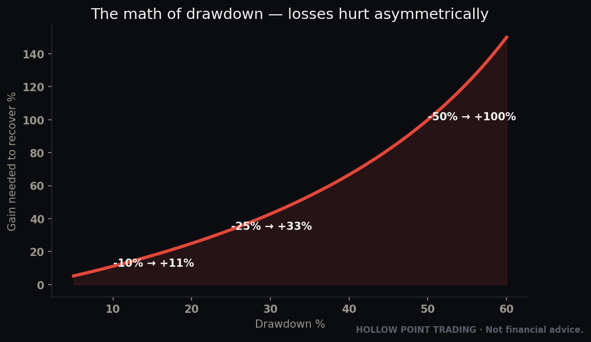
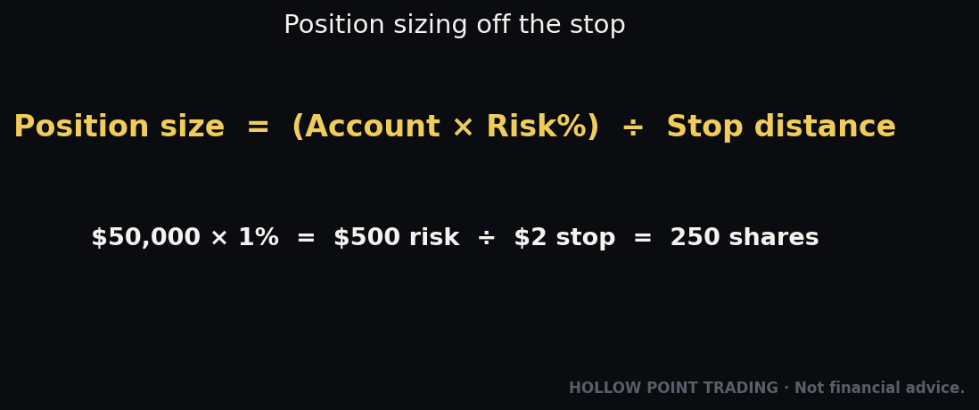
This is the real reason traders abandon good edges: not because the math failed, but because the drawdown that the math guarantees arrived and felt like the math had failed. If your position sizing can't survive eight consecutive −1R losses without emotional collapse or account damage, you will never be in the seat long enough to collect the +0.58R average. Expectancy tells you the destination. Variance tells you the size of the potholes on the way, and you must build the suspension to match. A concrete rule of thumb: risk per trade small enough that your worst plausible streak — roughly 8–10 losers for a 40% strategy — is an uncomfortable dent, never a crater. At 1R = 1% of account, ten straight losses is −10%: survivable, recoverable. At 1R = 5%, that same ordinary streak is −40%, and now you're a forced seller of your own edge at the worst possible moment.
How Regime Changes the Whole Picture
Here's something the textbook expectancy formula conveniently ignores: your edge is not a constant. The same setup has different expectancy in different market regimes, and lumping all regimes into one backtest number can hide a strategy that's a monster in one environment and a bleeder in another. Reading regime is half of reading expectancy.
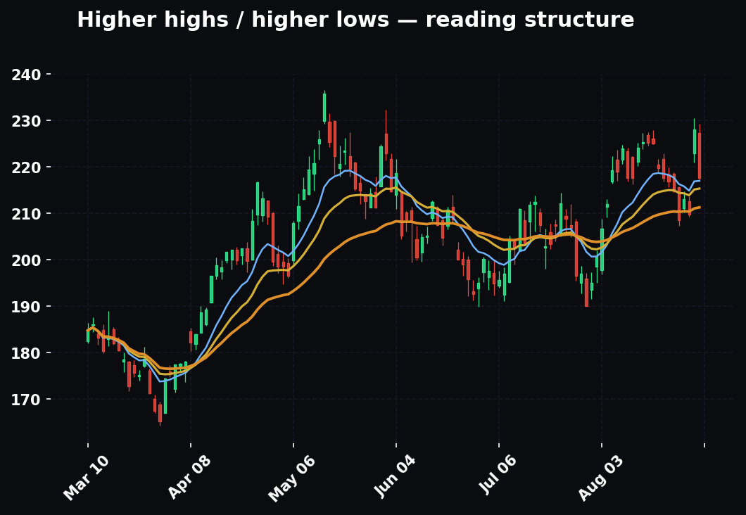
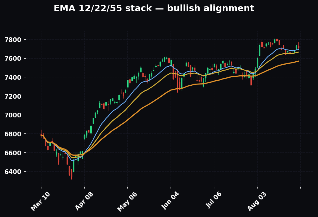
Trending regimes. Directional, breakout, and continuation setups — the 55-EMA reclaim, the opening-range break that runs, the pullback-to-trend entry — earn their keep here. Winners run further than your fixed target assumed, so your realized R:R often exceeds your planned R:R if you trail instead of capping. In a clean trend, a 40% setup can quietly become a 48% setup because failed breakouts are rarer when the tape actually wants to go. If your logged sample was gathered mostly in a trend, be honest that some of that expectancy is regime rent, not permanent edge.
Chop / range regimes. This is where trend-following setups go to die. Breakouts fail back into the range, reclaims get reclaimed the other way, and your win rate on directional setups can crater. That same 40% trend setup might print 25% in a two-week range — right at breakeven for a 1:3 — while mean-reversion setups (fade the range high, buy the range low) that lose money in a trend suddenly carry positive expectancy. The lesson isn't "trade the range setups instead." It's that your setup's expectancy has a regime dependency, and you should either measure it per-regime or throttle the setup down when its regime is absent. A trader who logs expectancy by regime learns to stand aside in chop instead of donating.
High-volatility regimes. Volatility widens everything: stops, targets, and slippage. Your fixed −1R stop gets hit more often on noise, dragging win rate down, but your winners are also bigger when they work. The dangerous part is the tails — gaps through stops, fills far from your intended price, and losers that come in at −1.4R instead of −1R because the market skipped your level. A backtest built in a calm regime will underestimate your average loss in a wild one. If you trade earnings weeks, CPI days, or a VIX-45 tape, your effective R:R is not what the calm-market backtest said. Either widen the stop and shrink the size to keep 1R constant in dollars, or don't take the setup until the regime normalizes.
The professional move is to tag every logged trade with its regime — trend up, trend down, range, high-vol — and compute expectancy per bucket. Nine times out of ten you'll discover your "edge" is really an edge in two regimes and a coin flip in a third. That single insight — trade the setup only in the regimes where it's proven — often adds more to your bottom line than any new setup ever will, because it converts your worst environment from a donation into a pass.
Multi-Timeframe Expectancy
Expectancy isn't a single number pinned to a setup — it's a number pinned to a setup on a timeframe, and the same pattern can carry wildly different edge depending on the clock you run it on. The 55-EMA reclaim on the 1-minute is a different animal from the same reclaim on the 15-minute, which is different again on the daily. They deserve separate logs and separate verdicts.
Two forces pull in opposite directions as you climb timeframes. Lower timeframes give you more trades — more repetitions, faster path to a large sample, quicker feedback on whether an edge is real. But they also carry worse signal-to-noise and heavier costs: spread and slippage are a fixed toll that eats a bigger fraction of a small target. A 1-minute scalp targeting 6 points on NQ pays the same commission and spread as a swing targeting 200 points, but that toll is a rounding error for the swing and a death sentence for the scalp if the gross edge is thin. Higher timeframes give you cleaner signal and fatter targets that swallow costs easily — but far fewer trades, so it takes months or years to gather a sample that clears the variance bar.
The practical framework is higher timeframe for bias, lower timeframe for the trade and the sample. The HPT thesis — that trades taken with higher-timeframe agreement outperform — is a claim about how one timeframe's context shifts another timeframe's expectancy. Test it directly: log your 15-minute reclaims in two buckets, one where the daily 55-EMA bias agreed and one where it didn't. If the higher-timeframe filter is real, the aligned bucket's expectancy is meaningfully higher. You're using the daily to raise the expectancy of the 15-minute trade, and now you can prove by how much. That's not a vibe about "confluence." That's a measured lift you can point to — the difference between, say, +0.58R aligned and +0.15R unaligned, which tells you in numbers to simply stop taking the unaligned version.
One trap to name: don't pool trades across timeframes into a single expectancy number. A blended "my reclaim setup is +0.4R" hides that the daily version is +0.9R and the 3-minute version is −0.1R after costs. Pooling averages a winner and a loser into a mediocre middle that describes neither, and worse, it can green-light the losing timeframe on the strength of the winning one. Separate logs, separate verdicts, always.
Confluence: Expectancy Alongside the Other Tools
Expectancy doesn't replace your read — it grades it. Here's how it interlocks with the tools you're already running, so it sharpens the top-down process instead of competing with it.
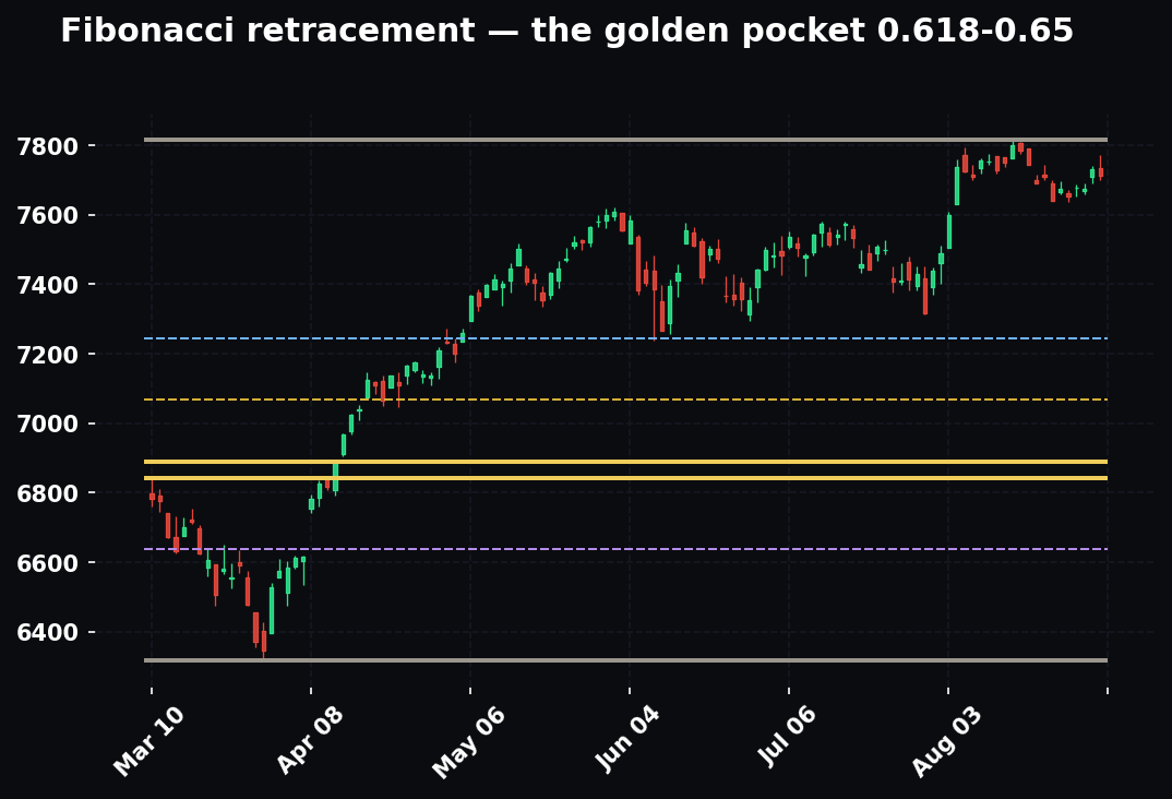
With the golden pocket (0.618–0.65 Fibonacci retracement). The golden pocket gives you a location — a high-probability zone to look for a reaction. Expectancy tells you whether reactions from that zone, on this setup, actually pay. Log your golden-pocket bounces as their own setup. You may find the pocket lifts your win rate by five points (better location = fewer noise stop-outs) and tightens your risk (stop just below the 0.65 keeps 1R small while target stays full), which compounds into a visibly higher expectancy than the same entry taken at a random pullback. The pocket earns its place in your process not because it looks elegant on a chart but because the logged expectancy of pocket-entries beats non-pocket entries. If it doesn't, the pocket is decoration for that setup, and the data just told you so.
With EMA structure (the 12/22/55 framework). The EMA stack defines regime and bias — price above a rising 55-EMA is a different world from price below a falling one. Use it as a filter that partitions your log. Trades taken with the stack aligned (entry above the 55 in an uptrend, momentum EMAs stacked in order) versus trades taken against it become two buckets. The near-universal finding when traders actually do this: the with-trend bucket carries the whole edge, and the counter-trend bucket is a coin flip or worse. That's the quantitative justification for "trade with the 55-EMA bias" — not dogma, a measured expectancy gap. It also tells you precisely which counter-trend scalps are worth keeping (the rare ones that clear the bar) and which to cut entirely.
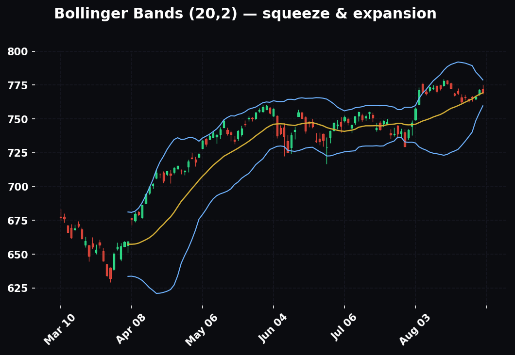
With volume / RSI as a confirming filter. Say you suspect that reclaims backed by above-average volume, or by RSI holding above 50, work better. Don't assume it — split the log and measure. This is where confluence turns dangerous, though, and it deserves a warning that belongs in the mistakes section too: every filter you add slices your sample smaller and invites curve-fitting. If "reclaim + volume > 1.5× + RSI > 50 + not-on-a-Monday" has beautiful expectancy over 18 trades, you haven't found confluence — you've fit noise. A confluence filter earns its keep only when it both raises expectancy and leaves you with a sample big enough to believe. The best confluence filters are few, logical, and each independently justified by a large-enough sub-sample — not a stack of six conditions tuned until the curve sparkles.
The unifying principle: your other tools generate location, bias, and confirmation. Expectancy is the scoreboard that tells you which combinations of those tools actually convert into money. Confluence without an expectancy test is a story. Confluence with one is an edge.
How to Read It and Use It: A Full Worked Evaluation
Let's put the whole machine together on a realistic setup. Say you trade the HPT 55-EMA reclaim on the 15-minute NQ: price loses the 55-EMA, reclaims it with a strong candle, you enter on the reclaim, stop below the reclaim low, target a defined 3R.
You go back through six months of charts and log every clean instance — not the ones you remember, every one that met the written rules. You get 120 trades. Here's the tally:
- Winners: 46 (reached +3R or you trailed to a comparable gain)
- Losers: 68 (stopped at −1R)
- Scratches: 6 (exited near breakeven, call them 0R)
Win rate (of decisive trades): 46 / 114 = 40.4%. Average win = +3R. Average loss = −1R. Fold the scratches in as 0R across all 120.
Expectancy = (46 × 3R) + (6 × 0R) + (68 × −1R), all divided by 120 trades = (138R + 0 − 68R) / 120 = 70R / 120 = +0.58R per trade.
Now read that like an analyst. 120 trades is a real sample — past the 100 threshold, into believable territory. The win rate is a coin-flip-ish 40%, which feels bad and is completely irrelevant, because the 3:1 R:R does the heavy lifting — remember, breakeven for a 1:3 is 25%, so 40% is a fat 15-point cushion above the line. Expectancy is +0.58R, comfortably above the +0.2R–0.3R "tradeable" line. If you risk $200 per trade (1R = $200), this setup has generated on average +$116 per trade over 120 trades. Take it 150 times a year and the expectancy is roughly $17,000 — assuming, and this is the whole ballgame, that you execute it exactly as tested.
Before you believe it, run the variance gut-check. Over 120 trades, the one-sigma swing on a 40% win rate is √(0.4×0.6/120) ≈ 4.5 points. So the true win rate is plausibly 36%–45%. Plug the pessimistic end into expectancy: (0.36 × 3R) − (0.64 × 1R) = 1.08 − 0.64 = +0.44R. Even in the unlucky-sample scenario, the edge stays clearly positive. That's a robust setup — one whose verdict survives the uncertainty in its own measurement. If the pessimistic end had flipped negative, you'd know the edge was too thin to trust on this sample and you'd need more data before sizing up.
A second worked example: the high-win-rate scalp
Now let's run a completely different animal so the machine's generality is clear. You also trade a VWAP-reversion scalp on the 3-minute: when price stretches a defined distance from VWAP and prints a rejection candle, you fade it back toward VWAP for a modest target. This is a high-win-rate, low-R:R setup — the mirror image of the reclaim.
You log 220 trades over three months (lower timeframe, so more instances):
- Winners: 143 at an average of +0.8R (you take profit at VWAP, a small target)
- Losers: 77 at an average of −1.0R (rejection fails, you're stopped)
Win rate = 143/220 = 65%. Expectancy = (0.65 × 0.8R) − (0.35 × 1.0R) = 0.52R − 0.35R = +0.17R per trade.
Read it honestly. The win rate is gorgeous — 65% feels like you can't lose. But the expectancy is only +0.17R, below the +0.2R–0.3R tradeable line. And we haven't touched costs yet. This is a 3-minute scalp with a small target, so spread and slippage bite hard. Say realistic costs are 0.1R per round trip (commission plus a tick of slippage on entry and exit). That drops every trade by 0.1R, taking expectancy to +0.07R — barely breathing. On this setup, the difference between "great win rate" and "actually worth trading" is entirely in the cost and the small R:R, and the gut-check is a warning, not a green light. The reclaim setup, with its ugly 40% win rate, is the far better business. That is the entire point of learning to read expectancy instead of win rate: it inverts the ranking your gut would give you.
Note also the sample logic. We needed 220 trades on the scalp partly because it's easy to get them (it fires often) and partly because a thin +0.07R edge needs a lot of confirmation before you'd trust it — a thin edge is exactly the kind that variance can fake into looking positive or negative. The fat +0.58R reclaim edge was believable at 120; the thin scalp edge isn't fully believable even at 220, and you'd want to see it hold across regimes before committing.
How It Fits the Top-Down Process
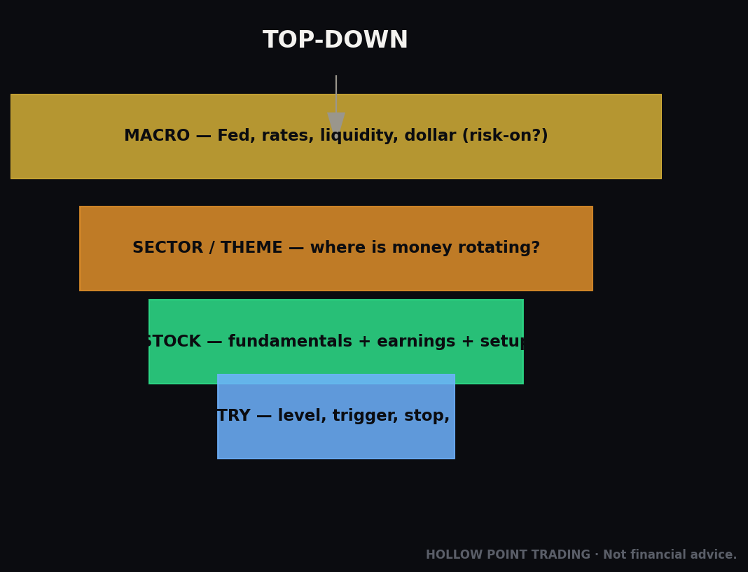
None of this replaces HPT's macro→sector→stock, timeframe-weighted framework — it arms it. Here's how expectancy threads into the top-down read instead of competing with it.
Top-down finds candidates; expectancy decides which ones earn size. The macro and sector work tells you where the wind is at your back — which names are in favorable regimes, which sectors are leading, where the higher-timeframe trend and the 55-EMA bias align. That's how you generate setups worth testing. Expectancy is how you rank them once you have them. You might trade five distinct setups; backtesting tells you which two carry real edge and which three you've been running on vibes.
Timeframe-weighted confluence should show up as higher expectancy — verify that it does. The HPT thesis is that trades taken with higher-timeframe agreement outperform. Good. That's a testable claim. Log your reclaim setups two ways: those where the daily 55-EMA bias agreed, and those where it didn't. Compute expectancy for each bucket. If confluence is real, the aligned bucket shows meaningfully higher expectancy — and now you have evidence for the filter, not just a belief. If it doesn't, the confluence rule isn't doing what you thought, and the data just saved you.
Position sizing lives downstream of a proven edge, never upstream. The 1:3 R/R rule and TF-weighted confluence set the shape of the trade. Expectancy proven over a real sample sets permission to size. The discipline HPT preaches — discipline over prediction — is precisely the refusal to increase risk on a setup whose edge you haven't earned the right to believe. You size up when the expectancy is positive and the sample is large enough that variance can't be the explanation. Not before. That single rule prevents most account-ending decisions.
Expectancy also tells you when to stop trading a setup.* The framework isn't only a gate for sizing up — it's a tripwire for sizing down. If a proven +0.58R setup starts printing −1R after −1R live and your rolling live expectancy drifts toward zero over a meaningful sample, that's data, not bad luck to push through. Either the regime that fed the edge has left, or your execution has drifted. The top-down process says: pull the setup back to minimum size, diagnose which of the two it is, and re-earn the permission before scaling back up. An edge is a lease, not a deed.
The Common Mistakes: Curve-Fitting and Its Cousins
Here is where good intentions go to die. Everything above assumes your backtest measured something real. Most don't. The failure modes are specific, they're seductive, and they all produce the same result: a beautiful backtest and a live account that bleeds. Here are the twelve that do the most damage, roughly in order of how often they wreck people.
1. Curve-fitting (overfitting). This is the big one. Curve-fitting is tuning a strategy so tightly to past data that it describes the noise of that specific history rather than any repeatable signal. You add a rule — "only take it if RSI is above 47.5 and volume is 1.8× average and it's a Tuesday" — and each rule makes the backtest prettier. It has to: with enough conditions you can perfectly describe any fixed set of past trades. But you've fit the coincidences of that exact history, and coincidences don't repeat. The tell is fragility: change 47.5 to 45 and the whole edge collapses. A real edge is robust — it survives small changes to its parameters, because it's capturing something the market actually does, not an accident of one dataset.
The defense: prefer few parameters over many. Prefer round, logical settings over precise magic numbers (a 50-EMA, not a 51.3-EMA). And demand that the edge hold across nearby parameter values — if +0.5R at a 55-EMA becomes −0.2R at a 50-EMA, you don't have an edge, you have a fit.
2. In-sample / out-of-sample failure. The clean way to catch curve-fitting: split your history in two. Build and tune the strategy on the first chunk — the in-sample data. Then test it, untouched, no more tweaking, on the second chunk it has never seen — the out-of-sample data. If expectancy holds up out-of-sample, you have real evidence. If it craters, you fit noise. The cardinal sin is peeking — tweaking the strategy after seeing out-of-sample results, which quietly turns your test data into training data and destroys the whole point. A stricter version the pros use is walk-forward: tune on months 1–3, test on month 4, roll forward, tune on 2–4, test on 5, and so on, so the test is always genuinely unseen and always adjacent in time.
3. Survivorship and hindsight bias. Backtesting only the setups you remember — the clean textbook ones — inflates everything. You have to log every instance the written rules produced, including the ugly ones you'd have talked yourself out of live. Related: hindsight makes past charts obvious. Standing at the hard right edge in real time, the setup was never as clean as it looks in the replay. This is why written, mechanical rules matter — they're the only thing that makes a backtest honest, because they remove your after-the-fact judgment from the count.
4. Ignoring costs and slippage. Commissions, spread, and slippage — the gap between the price you wanted and the price you got — quietly eat expectancy, and they hit high-frequency, small-R:R strategies hardest. A scalp showing +0.15R gross can be negative after costs, as our VWAP example nearly was. Bake realistic costs into every backtest. An edge that only exists in a frictionless world doesn't exist.
5. Confusing a lucky streak with an edge. The flip side of impatience. Ten green trades in a row is exactly what a positive-and a slightly-negative-expectancy strategy both produce sometimes. Don't let a hot streak promote a setup you haven't actually tested to real size. The math doesn't care how good you feel.
6. Abandoning a real edge during its guaranteed drawdown. The most expensive mistake on this list, and the mirror image of number 5. We showed that a 40% strategy will produce six-, seven-, even eight-loss streaks across a normal sample. Traders quit the good edge in the trough, right before the mean-reversion, then watch it rip without them. If you've done the variance work, a losing streak inside its expected range is confirmation the strategy is behaving normally, not evidence it broke. The only thing that should make you quit an edge is the expectancy going negative over a large fresh sample — never a streak that the math predicted.
7. Too many filters on too small a sample. Every condition you add to "improve" a setup carves your sample smaller. "Reclaim + volume + RSI + session + day-of-week" might leave you with 14 historical instances and a dazzling backtest that means absolutely nothing, because 14 trades is pure noise and five degrees of freedom can fit noise perfectly. Each filter must be justified by its own large-enough sub-sample, or it's just overfitting wearing the costume of confluence.
8. Moving the stop or target after entry. This silently changes the strategy you're measuring. You backtested a −1R stop and a +3R target. Live, you "give it room" and turn a −1R loss into −1.8R, or you take profit early at +1.2R because you're nervous. Now your realized R:R is nothing like the tested R:R, and your true expectancy is unknown and almost certainly worse. Discretion applied after entry doesn't just add risk — it invalidates your entire backtest, because you're no longer trading the thing you tested.
9. Regime blindness. Trading a trend setup in a range, or a calm-market setup through an earnings-week vol spike, and being shocked when the edge evaporates. As covered above: expectancy has a regime dependency. A backtest gathered in one regime overstates the edge in another. Tag your trades by regime or accept that your single blended number is lying to you about at least one environment.
10. Look-ahead bias in the backtest itself. A subtler cousin of hindsight: building rules that accidentally use information you wouldn't have had in real time. Entering "at the bar's close" but calculating the signal from the next bar's high, or using an indicator that repaints, or referencing a session's closing level to trade earlier in that same session. Any of these makes the backtest impossibly good and the live results impossibly bad. If a backtest looks too clean — near-100% win rate, no ugly stretches — suspect look-ahead before you celebrate.
11. Ignoring the tails and gap risk. Averages hide the killers. A strategy can have lovely expectancy and still contain a −6R overnight-gap disaster or a limit-down flash-crash fill lurking in its future that no calm backtest sampled. Expectancy is the center of the distribution; risk management is about the edges. Never let a good average lull you into position sizing that a single tail event can end. The average pays your bills; the tail closes your account if you let it.
12. Sample-mining across setups. Test twenty different setups and, by pure chance, two or three will show great backtested expectancy even if none has real edge — the same reason that if enough people flip coins, someone gets ten heads. If you go fishing across dozens of ideas and keep only the winners, you've selected for lucky noise. The discipline is to have a logical thesis for why a setup should work before you test it, so you're confirming a hypothesis rather than dredging a database for coincidences.
How the Pros Use It Differently From Beginners
The formula is the same for everyone. What separates a professional's use of it from a beginner's is almost entirely in the surrounding habits.
Beginners track one number; pros track a distribution. A beginner says "my setup is +0.4R." A pro knows the +0.4R is an estimate with a confidence band, knows the expected losing-streak length, knows the shape of the R-multiple distribution (a few fat winners carrying many small losers, or the reverse), and sizes for the drawdown, not the average. The average is where a beginner stops thinking and where a pro starts.
Beginners pool everything; pros segment obsessively. A pro doesn't have "an expectancy." They have expectancy by setup, by timeframe, by regime, by session, by day of week — enough segmentation to find where the edge lives and where it's being diluted, but not so much that any bucket falls below a believable sample. That segmentation is how a pro discovers that their overall breakeven strategy is actually a strong morning edge subsidizing a losing afternoon habit — and then simply stops trading the afternoon.
Beginners backtest to feel confident; pros backtest to try to kill the idea. A beginner runs the test hoping to confirm the setup works and stops the moment it looks good. A pro actively attacks their own strategy — nudges the parameters to check robustness, deducts pessimistic costs, isolates the worst regime, plugs the unlucky end of the variance band into the formula — trying to break the edge before the market does it with real money. A strategy that survives a genuine attempt to kill it is one you can size into. One that was only ever cheered for is one that will surprise you.
Beginners size by conviction; pros size by proven expectancy and drawdown tolerance. A beginner's size follows how good the trade feels — bigger when confident, which is exactly backwards, because conviction peaks right at tops and bottoms. A pro's size follows a formula: a fixed fraction of risk per trade, tuned to survive the strategy's expected worst streak, scaled up only when a large fresh sample confirms the edge is intact. Feeling is not an input to their position size. Ever.
Beginners chase win rate; pros engineer expectancy density. A beginner wants to be right. A pro wants total R per year — and knows that comes from expectancy per trade times frequency times the number of setups they can run in parallel without executional degradation. They'll happily trade an ugly 38%-win-rate setup that fires often and clears costs over a pretty 70% setup that barely beats the spread. Being right is a beginner's scoreboard. Total compounded R is a professional's.
Beginners treat the edge as permanent; pros treat it as decaying. Markets adapt; edges erode as more participants find them or as the regime that fed them passes. A pro monitors live expectancy against the backtested baseline continuously and expects to retire setups over time and replace them. A beginner finds one thing that worked in 2024 and is still forcing it, at size, long after the edge has bled out. The work is never finished; it's a rolling audit.
Frequently Asked Questions
Can expectancy be positive and I still lose money? Over a small sample, absolutely — variance can hand you a losing stretch even with a real edge, which is exactly why sample size and drawdown-survivable sizing matter. Over a large sample, if your live expectancy is genuinely positive and you execute the tested strategy, you make money; if you're still losing, either the live expectancy isn't actually positive (your backtest lied — costs, curve-fit, or regime) or your execution doesn't match the test.
How is expectancy different from profit factor? Profit factor is gross profit divided by gross loss — a ratio, above 1.0 means profitable. Expectancy is the average R (or dollars) per trade — a per-trade amount. They agree on whether you're profitable but expectancy is more useful for decisions, because it's per-trade and combines directly with frequency to tell you total expected R. Use expectancy as your primary; profit factor is a fine sanity cross-check.
What's a "good" expectancy number? In R terms, anything reliably above +0.2R to +0.3R per trade, held across a real sample and after costs, is a genuinely tradeable edge. Above +0.5R is strong. You do not need +1R or +2R monsters — those usually turn out to be small samples, curve-fits, or un-costed backtests. A modest, robust, repeatable positive beats a spectacular fragile one every time.
Do I really need 100+ trades? I don't get that many. Then you form opinions slowly and hold them lightly, which is the correct posture for a low-frequency trader. Options: test across more symbols that share the setup's logic (pooling comparable instances is legitimate), drop to a lower timeframe to gather more instances of the same pattern, or use replay to walk historical charts and log trades faster. What you must not do is declare victory at 12 trades because you're impatient — that's how you size up into noise.
Does forward-testing / paper trading really matter if my backtest is solid? Yes, because a backtest can't measure your execution or the current regime. Paper trading catches whether you can find and pull the trigger on the setup in real time without hindsight, whether your assumed fills are realistic now, and whether you follow the rules under pressure. Just remember paper fills are optimistic and paper pressure is zero — treat forward-test expectancy as a ceiling and re-confirm with small real size.
How do I handle a setup with wildly variable outcomes — some +1R, some +8R runners? Use the general expectancy formula (average of all trade R-multiples), not the two-bucket version, so the fat tails are counted at their real value. And be aware that fat-tailed, runner-driven edges need larger samples to trust, because so much of the total edge rides on catching the rare huge winners a representative number of times. A few missed monsters can make a great strategy look broken over a short window.
My backtested expectancy is +0.6R but live it's +0.1R. What happened? One of four things, and you diagnose them in order: (1) costs and slippage you didn't model — most common on lower timeframes; (2) execution drift — you're jumping entries, moving stops, or cutting winners, so you're trading a different, worse strategy than you tested; (3) regime change — the environment that fed the edge left; (4) the backtest was curve-fit or used look-ahead and the edge was never as big as it looked. Small real-size logging with honest notes usually reveals which within a couple dozen trades.
Should I stop a setup the moment expectancy dips? No — a dip within the strategy's known variance is expected and not actionable. You act only when live expectancy goes negative (or clearly below the backtest) over a fresh, meaningful sample, at which point you size down and diagnose rather than push through. The whole skill is distinguishing a normal drawdown the math predicted from a genuine regime or execution break. That distinction is what the variance work buys you.
The Cheat-Sheet
Print this. It's the whole guide compressed to what you'll actually reach for.
The formula. Expectancy = (Win% × Avg Win) − (Loss% × Avg Loss). Or, for messy real outcomes, just average every trade's R-multiple. Do it in R: 1R = your risk per trade. Positive = edge. Negative = no edge, regardless of feelings.
The breakeven line. Breakeven Win% = 1 / (1 + R:R). Memorize four: 1:1 needs 50%, 1:2 needs 33%, 1:3 needs 25%, 1:4 needs 20%. Any win rate above the line for your R:R makes money.
The verdict lines. Above +0.2R to +0.3R per trade, held over a real sample and after costs = tradeable edge. Above +0.5R = strong. Below 0 = stop trading it. You need a small repeatable positive, not a hero number.
Win rate ≠ edge. High win rate + tiny R:R can lose money (Trader A, 80% and broke). Low win rate + big R:R can print (Trader B, 35% and rich). Only expectancy decides. HPT's 1:3 R/R exists so a 40% win rate is plenty.
Expectancy density. Edge per trade × frequency = total R per year. A small edge you take often can beat a fat edge that rarely fires — if it survives costs.
Sample-size gates. <30 trades = noise, no opinion. 100+ = a real read. 200–300+ = confident, and mandatory for low-win-rate/high-R:R setups where rare winners carry the edge. To halve your uncertainty, quadruple your sample.
Variance gut-check. One-sigma win-rate swing ≈ √(p(1−p)/N). Small N = huge swings. Plug the pessimistic win rate into expectancy; if it stays positive, the edge is robust. Expect losing streaks the math guarantees — a 40% setup will hand you 6–8 straight losers in a normal sample. Size to survive them.
Regime. Tag every trade trend / range / high-vol and compute expectancy per bucket. Most "edges" are edges in two regimes and a coin flip in a third. Trade the setup only where it's proven; stand aside otherwise.
Timeframes. Separate log per timeframe — never pool. Higher TF for bias and clean signal and fat targets; lower TF for more trades and faster sample, but watch costs eat the small targets.
Curve-fit alarms. Many parameters, precise magic numbers, edge that collapses when you nudge a setting, a backtest that only counts the pretty setups, or filters stacked until a 14-trade sample sparkles. Prefer few round parameters; demand robustness across nearby values.
The honest test sequence. Logical thesis first → mechanical written rules → log every instance → split in-sample / out-of-sample (no peeking) → deduct real costs and slippage → forward-test live/small for dozens of trades → size up gradually while logging live expectancy vs backtest.
The one rule that saves accounts. Size up only when expectancy is positive and the sample is large enough that variance can't explain it and live execution matches the backtest. Not one of the three. All three.
Forward-Testing: The Bridge Between Backtest and Real Size
A backtest, however clean, is a measurement of the past. Forward-testing — also called paper trading — is running the strategy on live, unfolding data without risking real money, to see whether the edge survives contact with the present. It's the out-of-sample test that the future itself administers, and it catches things a historical backtest structurally cannot.
What forward-testing catches: whether you can actually find and execute the setup in real time, at the hard right edge, without hindsight; whether the current market regime still suits it; whether your fills are as good as you assumed; and whether you can follow the rules under live pressure. A strategy with +0.58R backtested expectancy is worth nothing if, live, you jump entries, move stops, and cut winners early — because now you're trading a different strategy than the one you tested, with an unknown and probably worse expectancy.
The honest progression, and the one HPT discipline demands, is a staircase, not a leap. Backtest to establish the edge exists historically. Forward-test on paper (or minimum size) for a meaningful sample — dozens of trades, not three — to confirm it survives live and that you can execute it. Then, and only then, size up gradually while you keep logging. At every step you're comparing live expectancy to backtested expectancy. If they match, press. If live is much worse, the problem is either regime change or you, and both need diagnosing before more size — not after.
One warning on paper trading: it removes the emotion, which is both its strength and its lie. Paper fills are optimistic and paper pressure is zero. Treat forward-test expectancy as a ceiling, not a promise, and confirm it again with small real size before you believe your own discipline holds when money is actually on the line. The gap between paper-you and real-money-you is where most "proven" strategies quietly die — not because the edge wasn't real, but because the person executing it became someone else the moment the P&L was live.
That's the machine. Win rate and R:R are the two dials. The breakeven line is the sanity check you do in your head. Expectancy folds the dials into a single verdict. Sample size and variance tell you when to believe that verdict — and how deep a drawdown you must be built to survive to collect it. Regime and timeframe tell you where the verdict applies. Forward-testing tells you whether it survives reality. And curve-fitting is the ghost that makes dead strategies look alive — the thing every one of these tools is really designed to exorcise.
Do this work on your top three setups and you'll likely find one is a genuine edge you've been under-trading, one is breakeven noise dressed up by a couple of memorable winners, and one you should have retired months ago. That's not a disappointment. That's the entire point — knowing, in numbers, which is which, before the market charges you tuition to find out.
Bound by rules, feared by trade.